5 Hydrological balance calculations
The first step to run the ERAHUMED DSS is to determine the system’s hydrology, as water serves as the primary transport medium for the chemicals under study. Specifically, by “hydrology,” we refer to the water volumes present in each water body at a given moment and the flow of water between them over a defined time frame (e.g., one day). Since most of these quantities are not directly measurable, they must be estimated through simulation. This Chapter outlines the algorithms used for this process.
5.1 Overview
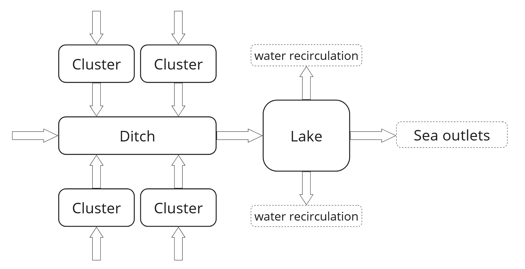
The hydrological module of ERAHUMED simulates the distribution and flow of water across the three main landscape elements of the Albufera Natural Park: the Albufera lake, rice field clusters, and irrigation ditches. This spatial representation was outlined in Section 2.2. For reference, we reproduce below the schematic diagram of the hydrogeographical model employed by ERAHUMED:
The overall simulation proceeds in three sequential steps:
Lake Hydrology
The water balance of the Albufera lake is computed first. Observed time series of lake water levels and outflows are combined with meteorological data on precipitation and evapotranspiration. The balance equation is used to estimate the unknown total inflow to the lake.Cluster Hydrology
Once the lake’s inflows are determined, the water balance of individual rice field clusters is simulated. Each cluster follows a water management plan defined by its assigned Rice Field Management System (RFMS), which specifies ideal irrigation and drainage schedules. The simulation adjusts real flows based on hydrological constraints, including shared ditch capacity.Ditch Hydrology
Finally, the hydrology of irrigation ditches is resolved. Under the simplifying assumption of constant ditch water levels, inflows and outflows are equated, and ditch inflows are estimated from the aggregated outflows of the clusters that drain into them.
5.2 Hydrology of the Albufera lake
Water balance calculations for the Albufera Lake are relatively simple. The relevant equation expressing hydrological balance is:
\[ \text{Volume Change} = \text{Inflow} - \text{Outflow} + \text{Precipitation} - \text{Evapotranspiration}. \tag{5.1}\]
The variables collected into the following table, that enter the balance equation 5.1, have direct correspondence with model input parameters listed in Chapter 3 (we use the notation df$col to indicate column col of data frame df).
| Variable | Source | Units | Description |
|---|---|---|---|
| \(h_t\) | outflows_df$level |
\(\text{m}\) | Lake water level daily time series |
| \(O_t^{\text{Pujol}}\) | outflows_df$outflow_pujol |
\(\text{m}^3\) | Pujol outflow daily time series |
| \(O_t^{\text{Perelló}}\) | outflows_df$outflow_perello |
\(\text{m}^3\) | Perelló outflow daily time series |
| \(O_t^{\text{Perellonet}}\) | outflows_df$outflow_perellonet |
\(\text{m}^3\) | Perellonet outflow daily time series |
| \(\text{P}_t\) | outflows_df$precipitation_mm |
\(\text{mm}\) | Precipitation (per unit area) daily time series |
| \(\text{ET}_t\) | outflows_df$evapotranspiration_mm |
\(\text{mm}\) | Evapotranspiration (per unit area) daily time series |
| \(\alpha\) | storage_curve_intercept_m3 |
\(\text{m}^3\) | Storage curve intercept |
| \(\beta\) | storage_curve_slope_m2 |
\(\text{m}^2\) | Storage curve slope |
| \(\sigma _\text{PET}\) | petp_surface_m2 |
\(\text{m}^2\) | PET surface |
Calculated quantities are listed in the following table.
| Variable | Units | Description |
|---|---|---|
| \(V_t\) | \(\text{m}^3\) | Lake water volume daily time series |
| \(\Delta V_t \equiv V_{t+1}-V_t\) | \(\text{m}^3\) | Lake water volume change daily time series |
| \(\Delta V_t^{\text{PET}}\) | \(\text{m}^3\) | Lake water volume change due to precipitation and evapotranspiration daily time series |
| \(I_t\) | \(\text{m}^3\) | Lake total inflow daily time series |
| \(O_t\) | \(\text{m}^3\) | Lake total outflow daily time series |
The volume time-series is computed as:
\[ V_t = \alpha + \beta \cdot h_t, \tag{5.2}\]
while the volume changes due to precipitation and evapotranspiration are given by:
\[ \Delta V_t ^{\text{PET}} = \sigma _{\text{PET}}(\text{P}_t - \text{ET}_t), \tag{5.3}\]
Total inflow and outflow must satisfy Equation 5.1, which we may rewrite explicitly as:
\[ \Delta V_{t} -\Delta V^{\text{PET}}_t = I_t - O_t, \tag{5.4}\]
Strictly speaking, \(O_t\) is not merely the sum of \(O_t^{\text{Pujol}}\), \(O_t^{\text{Perelló}}\) and \(O_t^{\text{Perellonet}}\), but is rather calculated as follows:
\[ O_t = \max \left[ O_t^{\text{Pujol}} + O_t^{\text{Perelló}} + O_t^{\text{Perellonet}},\, \Delta V^{\text{PET}}_t -\Delta V_{t} \right]. \tag{5.5}\]
The rationale is that the simple sum of estuaries outflows omits potentially important contributions from water recirculation, that is to say, water being pumped out from the lake for rice-field irrigation, by the so-called tancats. Such amount of recirculated water is hard to estimate and, in the lack of a better model, we simply assume this to be negligible, except when a positive amount is required by Equation 5.4 itself, due the physical constraint that \(I_t \geq 0\).
Once \(O_t\) is calculated through Equation 5.5, \(I_t\) can be immediately obtained from Equation 5.4. Notice that whenever the aforementioned compensating outflow term due to water recirculation is included (which happens when the maximum in Eq. 5.5 is given by the second term), the total inflow is always estimated to be zero.
5.3 Hydrology of rice field clusters
Water balance calculations for rice field clusters are complex due to the lack of observational data. The simulation algorithm relies on several key components:
- The hydrology of the Albufera lake (Section 5.2).
- Assumptions about the hydrological connections between the various water bodies in the natural park, detailed in Section 2.2.
- An ideal yearly management plan for irrigation and drainage of rice field clusters, that depends on the management systems employed by individual clusters. The details of this derivation are described in Chapter 4.
The quantitative inputs for this calculation are collected in the following table; the ideal irrigation/draining schedules and water levels are calculated as described in Section 4.2 and are specific to the RFMS assigned to the cluster under study.
| Variable | Source | Units | Description |
|---|---|---|---|
| \(\text{Ir}_{d,c}\) | See text | \(\text{NA}\) | Boolean expressing whether cluster \(c\) is supposed to be irrigated on day of year \(d\) |
| \(\text{Dr}_{d,c}\) | See text | \(\text{NA}\) | Boolean expressing whether cluster \(c\) is supposed to be drained on day of year \(d\) |
| \(\mathcal H _{d,c}\) | See text | \(\text{cm}\) | Ideal water depth (in \(\text{cm}\)) of cluster \(c\) on day of year \(d\) |
| \(k_\text{flow}\) | ideal_flow_rate_cm |
\(\text{cm}\cdot \text{day} ^{-1}\) | Rate of water flow through rice paddies during simultaneous irrigation and drainage, while maintaining a constant overall water level. |
| \(h_{\text{thres}}\) | height_thresh_cm |
\(\text{cm}\) | Water height below which a cluster is considered emptied. Used to determine delays in the draining/irrigation plan. Expressed in \(\text{cm}\). |
| \(A_c\) | Internal parameter | \(\text{m}^2\) | Surface area of cluster \(c\) |
The outputs are collected below, where the indices \(c\) and \(t\) denotes the cluster and time, respectively:
| Variable | Units | Description |
|---|---|---|
| \(V_{c,t}\) | \(\text{m}^3\) | Cluster’s water volume |
| \(I_{c,t}\) | \(\text{m}^3\) | Cluster’s inflow |
| \(O_{c,t}\) | \(\text{m}^3\) | Cluster’s outflow |
The fundamental equation for hydrological balance is:
\[ V_{c,t+1}-V_{c,t} = I_{c,t}-O_{c,t} + (\text{P}_t-\text{ETP}_t)\times A_c \tag{5.6}\]
where \(\text{P}_t\) and \(\text{ETP}_t\) are the same as in Section 5.2.
In what follows, we will focus on the set of all clusters draining into a given ditch, and we will enumerate clusters through the index \(c = 1,\,2,\,\dots,\,N_C\). On the other hand, clusters are assumed to be irrigated from sources external the Albufera system, i.e., not through any of the ditches that eventually flow into the lake. According to our assumptions on the hydrology of clusters and ditches (cf. Section 2.2), the sum of cluster outflows is constrained by:
\[ \sum _{c = 1} ^ {N_C} O_{c,t} \leq Q_t \tag{5.7}\]
where \(Q_t\) denotes the inflow to the relevant ditch. With a small leap in logic, we anticipate from Section 5.4, that the water levels in irrigation ditches are assumed to be constant, so that \(Q_t\) can also be identified with the ditch outflow, that is in turn estimated as:
\[ Q_t = \frac{\text{Area of clusters draining into ditch}}{\text{Area of all clusters}} \times \text{Lake's Inflow}_t \tag{5.8}\]
where the lake’s inflow is computed as described in Section 5.2.
Qualitatively speaking, the simulation determines daily values of \(I_{c,t}\) and \(O_{c,t}\) that satisfy Eqs. 5.6 and 5.7, and such that the resulting hydrology aligns as closely as possible with the “ideal” conditions prescribed by the specified management plan. This is accomplished in three steps:
- Computing ideal inflows and outflows based on current water levels and management plans.
- Determining actual inflows and outflows, along with the corresponding actual water level changes.
- Adjusting management plan delays if some clusters were scheduled to be drained but could not be due to insufficient flow through the common ditch (see below for details).
These steps are iterated on a daily basis, starting from some initial time (say \(t = 0\)) at which all cluster water levels match the ideal ones, and no plan delays are present.
Concerning the last step, a few words may serve to clarify the algorithm described below. The purpose of management plan delays is to ensure that during each year’s sowing season, all cluster’s are eventually emptied as required for ground applications of chemicals (modeled in subsequent layers of the simulation). This is achieved by postponing the management plan by one day whenever an emptying condition is not met. Outside of the sowing window, delays are reset to zero to prevent them from accumulating indefinitely, which would be unrealistic.
In what follows, the conversion between cluster water volumes and depths is provided by \(V_{c,t} = A_c \cdot h_{c,t}\), and we denote by \(\delta_{c,t}\) the time series of plan delays for cluster \(c\), which is initialized by \(\delta_{c,0} =0\).
5.3.1 Step 1: ideal balance
Ideal balance quantities for each cluster \(c\) are obtained from the ideal water management variables \(\text{Ir}_{d,c}\), \(\text{Dr}_{d,c}\) and \(\mathcal H _{d,c}\), by matching the day of year \(d\) with the delayed day:
\[ d_{c,t+1} = d_{t+1}-\delta_{c,t}, \tag{5.9}\]
where \(d_{t+1}\) denotes the day of year corresponding to time \(t+1\), and \(\delta_{c,t}\) the accumulated plan delay.
Let \(h _{c,t+1}^{\text{id}}\) denote the ideal depth for cluster \(c\) at time \(t+1\) retrieved in this way, and \(\text{Ir}_{c,t}\), \(\text{Dr}_{c,t}\) the corresponding irrigation and draining plans. Furthermore, denote by \(V_{c,t+1}^{\text{id}} = A_c \cdot h_{c,t+1}^{\text{id}}\) the corresponding ideal water volume.
In order to compute ideal inflow and outflow, we require (cf. Equation 5.6):
\[ V_{c,t+1}^{\text{id}} = \max \lbrace V_{c,t}^{\text{id}} + (\text{P}_t-\text{ETP}_t)\times A_c,0 \rbrace + I_{c,t}^{\text{id}}-O_{c,t}^{\text{id}} \tag{5.10}\]
Clearly, Equation 5.10 alone does not individually specify \(I_{c,t}^{\text{id}}\) and \(O_{c,t}^{\text{id}}\), but only their difference \(\Delta _{c,t}^{\text{id}}= I_{c,t}^{\text{id}}-O_{c,t}^{\text{id}}\). In order to fix both these quantities:
\[ \begin{split} (I_{c,t} ^\text{id})^{(0)}&= \begin{cases} k_\text{flow} & \text{if }\text{Ir}_{c,t} = \text{Dr}_{c,t} = 1 \\ 0 & \text{otherwise} \end{cases},\\ (O_{c,t} ^\text{id})^{(0)}&=(I_{c,t} ^\text{id})^{(0)}-\Delta _{c,t}^{\text{id}}. \end{split} \tag{5.11}\]
and, in order to ensure that flows are positive, we finally set:
\[ \begin{split} O_{c,t} ^\text{id} &= \max\lbrace(O_{c,t} ^\text{id})^{(0)},\,0\rbrace\\ I_{c,t} ^\text{id} &= O_{c,t} ^\text{id} + \Delta _{c,t}^{\text{id}}, \end{split} \tag{5.12}\]
which satisfy Equation 5.10 and give rise to positive \(O_{c,t}^\text{id}\) and \(I_{c,t}^\text{id}\).
5.3.2 Step 2: real balance
At each time-step \(t\), the cluster’s index set is randomly permuted 1, and the real flows are calculated as:
\[ \begin{split} O_{c,t} &= \min \lbrace O_{c,t}^\text{id},\,Q_t-\sum_{c'<c}O_{c',t} \rbrace ,\\ I_{c,t} &= \max\lbrace I_{c,t}^\text{id}-O_{c,t}^\text{id} + O_{c,t},\,0 \rbrace \end{split} \tag{5.13}\]
In simple terms, clusters are emptied in a random order within the allowed capacity of the corresponding ditch. Using Equation 5.13, we finally determine the real water level achieved as:
\[ V_{c,t+1} = \max \lbrace V_{c,t} + (\text{P}_t-\text{ETP}_t)\times A_c,0 \rbrace + I_{c,t}-O_{c,t} \tag{5.14}\]
to be compared with Equation 5.10.
5.3.3 Step 3: updating the plan delay
The updated value \(\delta _{c,t+1}\) is obtained as follows. If \(d_{t+1}\) (the actual day of year) is outside of the window \([\text{Sowing day},\,\text{Start of Perellonà}]\) (which is specified by the RFMS assigned to cluster \(c\), see Section 4.2), then \(\delta_{c,t+1} = 0\). Otherwise, if \(h_{c,t}^\text{id} > 0\) or \(h_{c,t} < h_{\text{thres}}\), the plan delay is unchanged: \(\delta_{c,t+1} = \delta_{c,t}\). Finally, if \(h_{c,t}^\text{id} = 0\) but \(h_{c,t} > h_{\text{thres}}\), we add one day of delay: \(\delta_{c,t+1} = \delta_{c,t}+1\).
5.4 Hydrology of irrigation ditches
Our approach to the hydrology of irrigation ditches is simplified, with the main assumption being that all ditches have a common, constant water depth \(h_\text{ditch}\) corresponding to the input parameter ditch_level_m.
Using the index \(D =1,2,\dots,26\) to enumerate the park’s main ditches, ditch outflows to the Albufera lake \(O_{D,t}\) are calculated according to Equation 5.8. These outflows also coincide with the total ditch inflows \(I_{D,t}\) (due to the constant water volume assumption).
With some abuse of notation, we assume the indexes \(c\) and \(c'\) in Equation 5.13 to be sorted according to this random permutation.↩︎