6 Exposure
This Chapter describes how the ERAHUMED DSS models pesticide exposure in the water and sediment of the water bodies of the Albufera Natural Park. The hydrological simulation discussed in the previous Chapter provides the foundation for this analysis, as water serves as the primary medium for pesticide transport. Here, we outline how ERAHUMED simulates the introduction, dispersion, and fate of pesticides within the system. This includes processes such as deposition, degradation, and transfer between water bodies. By integrating hydrological dynamics with chemical fate and transport, the model estimates exposure levels over time and space.
The conceptual representation of pesticide fate and transport processes in ERAHUMED considers some of the processes included in the RiceWQ model by Williams et al. (2004) (developed by the International Rice Research Institute and Wageningen University). At the cluster level, the ERAHUMED builds upon the conceptual framework of RiceWQ, adapting it to the ecological and hydrological context of the Albufera Natural Park. In doing so, it introduces an efficient semi-analytic solution of the governing equations and is released as open-source software.
As illustrated in our hydrological model (Figure 2.2), pesticides applied to rice field clusters are transported through water flow into ditches, then into the Albufera lake, and ultimately to the sea.
From a mathematical perspective, the fate of chemicals in each water body—clusters, ditches, and the lake—is governed by the same system of differential equations. These equations represent key physico-chemical processes, including advective transport, diffusive exchange between compartments, and degradation. However, pesticide applications occur exclusively in clusters; concentrations in ditches and the lake arise solely from upstream inflows.
The remainder of this chapter describes our approach to pesticide dispersion. We define the simplified differential system used to model these processes in Section 6.2, and we present our semi-analytic solution method in Section 6.3. Section 6.4 finally describes how the parameters of the differential system are derived from the basic input parameters listed in Chapter 3.
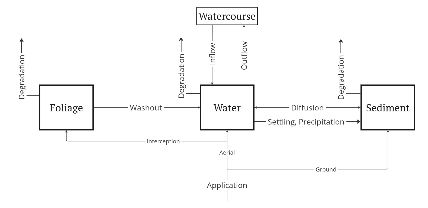
6.1 Diagram of physical processes
The schematic diagram below illustrates the processes captured by our model for chemical dispersion. Directional arrows represent the transfer of chemical matter among the three compartments considered—Foliage, Water, and Soil—as well as exchanges with external water bodies (denoted as “Watercourse”).
While the overall scheme applies to all landscape elements, specific details vary for clusters, ditches, and the lake (cf. the hydrological model of Figure 2.2):
- Clusters: Inflow waters originate outside the system and are assumed to be free of pesticides.
- Ditches and the Albufera lake: No direct pesticide applications occur in these areas, meaning the foliage compartment plays no role in their dynamics.
- Ditches: Receive inflows from two sources—clusters, which contribute pesticide-laden water, and external sources, which are assumed to be free of chemicals.
- Albufera lake: Its only inflows come from ditches, which contain nonzero chemical concentrations.
6.2 Evolution Equations
We focus on a single pesticide and a fixed hydrological element (e.g., a cluster). We denote its masses in the three compartments—foliage1, water, and sediment—by \(m_f\), \(m_w\), and \(m_s\), respectively. We assume that, at any given time, these masses are fully diluted and homogeneously distributed. In particular, we can meaningfully define spatially constant concentrations \(c_f\) and \(c_s\) in the water2 and sediment compartments.
We provide below the differential system that drives the temporal dynamics of \(m_f\), \(m_w\) and \(m_s\). The correspondence between the parameters used in this Section and the ERAHUMED model inputs is provided later (Section 6.4).
The fundamental equations describing pesticide diffusion are given as follows:
\[ \begin{split} \dfrac{\text d{m}_f}{\text d t} & = -(k_f+w)m_f+a_f\\ \dfrac{\text d{m}_w}{\text d t} & = -(k_w+d_w+s+\frac{O}{V})m_w+d_sm_s+wm_f+a_w-\sigma(\frac{m_w}{\rho V}) \\ \dfrac{\text d{m}_s}{\text d t} & = (d_w+s)m_w-(k_s+d_s)m_s+a_s+\sigma(\frac{m_w}{\rho V}) \end{split} \tag{6.1}\]
where:
- \(a_{f,w,s}\) are the mass income rates of the chemical in the three compartments, that include direct pesticide application and mass coming from inflows.
- \(k_{f,w,s}\) are the degradation rates of the chemical in the three compartments,
- \(d_w\) and \(d_s\) are the water-sediment diffusion rates,
- \(s\) is the settling rate,
- \(w\) is the washout rate,
- \(O\) is the outflow rate of the rice field,
- \(V\) is the volume of water in the rice field,
- \(\rho\) is the chemical solubility in water,
- \(\sigma(x)\) is a function (not further specified, see below) that grows quickly for \(x > 1\), and vanishes for \(x \leq 1\). This function accounts for solubility.
Strictly speaking, all these terms have instantaneous time dependence3. Apart from making the system 6.1 hard to attack by analytic means, such a dependence is troubling because we don’t have access to the exact time dependence of the majority of these terms (e.g. outflow, volume or chemical applications), our input consisting of simple daily average/cumulative values. On the other hand, if all the terms were constant, and if we could neglect \(\sigma\), the solution of Equation 6.1 would be immediate, as the corresponding system becomes a linear Ordinary Differential Equation (ODE) with constant coefficients, in addition whose eigenvalues and eigenvectors can be computed explicitly.
What we use in practice is an intermediate semi-analytic approach that allows us to compute daily values of \(m_{f,w,s}\), which is described next.
6.3 Semi-analytic solution of Equation 6.1
The time evolution of \(m_{f,w,s}\) in a daily time-step (from \(t\) to \(t+1\), say, assuming \(t\) is measured in days) is obtained through the following four consecutive stages:
- We compute the exact evolution of \(m_{f,w,s}\) according to the linear ODE obtained by disregarding the processes of outflow, chemical application and solubility, and using daily constant values for all the remaining constants involved (described in more detail below).
- We compute the \(m_w\) losses due to outflow as if they happened instantaneously after the processes computed in the previous step took place, with the water volume of the rice paddy varying from \(V(t+1)+O(t)\) to \(V(t+1)\).
- We compute the mass applications again as instantaneous, after the losses in the water compartment due to outflows took place.
- We compare the resulting \(m_w\) with the maximum amount allowed by the solubility in water, that is \(m_w ^{\text{max}}(t) = \rho V(t+1)\) and transfer any excess to the sediment compartment (\(m_s\)).
In the following, we describe in full detail the computations involved in these four steps.
6.3.1 Step 1: linear ODE evolution (physico-chemical processes)
Disregarding outflow, mass application and solubility, we get a linear ODE of the form:
\[ \begin{split} \dfrac{\text d{m}_f}{\text d t} & = \gamma m_f,\\ \dfrac{\text d{m}_w}{\text d t} & = a_{ww} m_w+a_{ws}m_s + w m_f, \\ \dfrac{\text d{m}_s}{\text d t} & = a_{sw}m_w+a_{ss}m_s, \end{split} \tag{6.2}\]
with:
\[ \begin{split} \gamma &= -(k_f + w),\\ a_{ww} &= - (k_w + d_ w +s)\\ a_{ws} &= d_s\\ a_{sw} &= d_w+s\\ a_{ss} &= -(k_s+d_s) \end{split} \tag{6.3}\]
where the various physico-chemical parameters are assumed to be constant during a daily time-step (cf. Section 6.4).
The evolution of \(m_f\) is easily obtained:
\[ m_f(t) = e^{\gamma t}m_f(0). \tag{6.4}\]
Plugging this into the three-dimensional system 6.2 we obtain a reduced two-dimensional system for the water-sediment compartments:
\[ \begin{split} \dfrac{\text d{m}_w}{\text d t} & = a_{ww} m_w+a_{ws}m_s + w e ^{\gamma t}m_f(0), \\ \dfrac{\text d{m}_s}{\text d t} & = a_{sw}m_w+a_{ss}m_s, \end{split} \tag{6.5}\]
which is solved explicitly with standard methods4.
6.3.2 Step 2: mass losses due to outflow
Mass losses due to outflow are computed as if the outflow process happened instantaneously after the processes discussed in the previous step took place. The amount of mass in the water compartment is affected as follows:
\[ m_w \to \frac{V_f}{V_i} m_w, \tag{6.6}\]
where \(V_i\) and \(V_f\) denote the initial and final volume for the outflow process. Here \(V_f\) coincides with the simulated value \(V(t+1)\) for the relevant water body and \(V_i = V_f + O(t)\), where \(O(t)\) denotes the total simulated outflow for day \(t\).
6.3.3 Step 3: mass income from direct application and inflows
These contributions are computed as instantaneous and subsequent to outflow. Masses in the various compartments (\(i = f,\,w,\,s\)) are modified as follows: \[ m_i \to m_i + a_i \tag{6.7}\]
As mentioned above, \(a_i\) accounts for both direct pesticide applications and water inflow, that is:
\[ a_i = a_i ^{\text{app}} + a_i ^{\text{inflow}} \]
The calculation of direct application rates from input parameters is described below. As to the second term, the amount of incoming mass is exactly given by the amount of outgoing mass in the outflow of the preceding element along the water course chain, which is computed as detailed in the previous Section.
6.3.4 Step 4: solubility
The chemical density in the water compartment after Steps 1, 2, and 3 is eventually compared with the chemical’s solubility \(\rho\), and any mass excess is instantaneously transferred to the sediment compartment. This implies the following modifications:
\[ m_s \to m_s + \max(0, \,m_w - \rho V(t+1)),\quad m_w\to\max(m_w,\,\rho V(t+1)). \tag{6.8}\]
6.4 Input parameters (correspondence with Chapter 3)
This section describes the sources of the numerical inputs to Equation 6.1, highlighting their correspondence with the parameters listed in the tables of Chapter 3.
6.4.1 Mass income rates
Mass input to water elements arises from two sources: direct application and transport via inflow. Accordingly, we can express the total mass input as:
\[ a_X = a_X ^{\text{app}}+ a_X ^{\text{inflow}} \qquad (X = f,\,s,\,w). \tag{6.9}\]
where \(X\) denotes the compartment receiving the input.
The inflow contribution is computed as:
\[ a_X ^{\text{inflow}} = \sum _{i} m_i ^{\text {inflow}}, \tag{6.10}\]
where the sum runs over the relevant inflow sources for the water body under consideration. Inflow masses \(m_i ^{\text {inflow}}\) Equation 6.6 are obtained from Equation 6.6 when the source is a hydrological element higher in the flow network (e.g., clusters for ditches, or ditches for the lake). At the current stage of development, external sources are assumed to have zero pesticide concentration and are thus excluded from the mass inflow calculation.
Application rates are given by:
\[ \begin{split} a_f^{\text{app}} &= A(t)\cdot \phi(t),\\ a_s^{\text{app}} &= A(t)(1-\phi(t))I(h(t+1)=0),\\ a_w^{\text{app}} &= A(t)\cdot (1-\phi(t))I(h(t+1)\neq0),\\ \end{split} \]
Here, \(A(t)\) is the applied amount on day \(t\), whose computation is described below; \(I(h(t+1)=0)\) is equal to one if the water level of the cluster \(h(t+1) =0\), and vanishes otherwise5; the quantities \(\text{drift}\), \(\text{SNK}\) correspond to the internal drift and SNK parameters (cf. Chapter 3); finally \(c\) is the coverage fraction, computed as:
\[
\phi(t) = \min\left[\frac{d_s(t)}{j_{\text{grow}}},\,1\right]\cdot \phi_{\text{max}},
\] where \(d_s(t)\) is the number of days elapsed from seeding, while \(j_\text{grow}\) and \(\phi_\text{max}\) correspond to the input parameters jgrow and covmax.
The actual day on which a pesticide application takes place is determined by adjusting the nominal application day specified in the RFMS definition (see Section 4.2) using the plan delay computed in the hydrological simulation (see Section 5.3). Concretely, if we denote by \(\mathcal D\) the nominal day of year for pesticide application, by \(d_{t}\) the day of year corresponding to a given date \(t\), and by \(\delta _{c,t}\) the plan delay for a cluster \(c\) on the same date (cf. Equation 5.9), the actual application date6 is given by:
\[ T_{\text{application}} =\max\lbrace t \,\vert\, d_{t}-\delta_{c,t} = \mathcal D\rbrace \tag{6.11}\]
The amount of active ingredient applied is defined by the corresponding dose parameter in the input specification (cf. Table 3.4).
6.4.2 Degradation rates
Daily degradation rates \(k_{f,w,s}(t)\) for the chemical are modeled through the Arrhenius equation, schematically:
\[
k(t) = k_0 \cdot Q_{10}^{\frac{T(t)-T_0}{10}}
\] where \(k_0\) is the degradation rate \(k_0\) at a reference temperature \(T_0\), \(Q_{10}\) is a numerical constant, and \(T(t)\) is the average temperature on day \(t\). All these numerical quantities are chemical input parameters (see Table 3.2), except for the daily temperature \(T(t)\), that comes from observational data (column temperature_ave of weather_df, see Section 3.1.1.1 for reference).
For the sediment compartment, we compute two degradation constants \(k_s^{\text{sat/unsat}}\), for saturated and unsaturated sediment, respectively (the input parameters for the calculation of these two constants are independent, see Table 3.2). The degradation rate in the solid compartment at time \(t\) is eventually given by:
\[ k_s(t) = k_s ^{\text{sat}}(t) I(h(t)\neq0)+k_s ^{\text{unsat}}(t) I(h(t)=0) \tag{6.12}\]
6.4.3 Diffusion rates
Diffusion rates are given by:
\[
d_w(t) = \frac{k_\text{dif}\cdot f_{D,w}}{h(t)}, \quad d_s = \frac{k_\text{dif}\cdot f_{D,s}}{h_{\text{act}}\cdot \text{pos}}
\] where \(h(t)\) is the water depth of the hydrological element; \(h_\text{act}\) is the depth of active sediment, corresponding to the simulation parameter dact_m; \(\text{pos}\) corresponds to the porosity simulation parameter; \(k_\text{dif}\) is given by the empirical formula:
\[ k_\text{dif} = \left( \frac{69.35}{365} - \text{pos}\cdot M^{-2/3} \right)\frac{\text{m}}{\text{day}} \]
where \(M\) is the molecular weight of the chemical (chemical parameter MW); finally, \(f_{D,w}\) and \(f_{D,s}\) are given by:
\[ f_{D,w} = \frac{1}{1+c^{\text{ss}}\cdot k_d^{\text{ss}} } \qquad f_{D,s} = \frac{\text{pos}}{\text{pos}+b_d\cdot k_d^{\text{sed}} } \qquad \]
where \(c^{\text{ss}}\) and \(b_d\) correspond to the input parameters css_ppm and bd_g_cm3, while \(k_d^{\text{sed/ss}}\) are the partition sediment and suspended solid water partition coefficients, computed as:
\[
k_d ^{\text{sed/ss}} = \text{foc}^{\text{sed/ss}}\cdot k_\text{oc}
\] where \(\text{foc}^{\text{sed/ss}}\) correspond to the environmental parameters foc_ss and foc_sed, respectively, and \(k_\text{oc}\) is the chemical parameter koc_cm3_g.
6.4.4 Settling rate
The daily settling rate is computed as:
\[
s(t) = \dfrac{k_{\text{setl}}(1-f_{D,w})}{h(t)}
\] where \(k_{\text{setl}}\) corresponds to the chemical parameter k_setl_m_day.
6.4.5 Washout rate
The daily washout rate is computed as:
\[
w(t) = \text{fet} \cdot P(t)
\] where \(P(t)\) is the daily precipitation per unit area, while \(\text{fet}\) is the chemical parameter fet_cm.
6.4.6 Solubility
The solubility \(\rho\) of chemicals correspond to the solubility input parameter.
The foliage compartment is only relevant for rice field clusters, as direct application is the only mechanism through which pesticides reach plant surfaces. Ditches and the lake do not receive foliar pesticide inputs.↩︎
Provided the water volume is nonzero.↩︎
This observation also includes pure physico-chemical “constants” such as degradation rates, where the time dependence would stem from temperature dependence.↩︎
Letting \(x = (m_w,\,m_s)^T\) and \(b = w(m_f(0),0)^T\), the system can be rewritten in the form: \[ \dot x = Ax + e^{\gamma t }b \] where \[ A = \begin{pmatrix} a_{ww} & a_{ws} \\ a_{sw} & a_{ss} \end{pmatrix} \] The general solution reads: \[ x(t) = e^{At}x(0)+(e^{At}-e^{\gamma t}I)(A-\gamma I)^{-1}b \] where \(I\) is the identity matrix. Notice that the exponential can be computed explicitly from the eigenvalues of \(A\): \[ e^{At} = e^{\lambda _+ t} P_+ + e^{\lambda _- t} P_-, \] with: \[ \lambda _{\pm} = \frac{\text{Tr}A}{2} \sqrt{\left(\frac{\text{Tr}A}{2}\right)^2 - \det A} \] and \[ P_{\pm} = \pm \frac{1}{\lambda _+ - \lambda _-}(A-\lambda _{\mp}) \]↩︎
The reason why the height of day \(t+1\) is used here is because, as mentioned above, applications are computed using the final water volume of the cluster, as if all daily water flows already took place.↩︎
For simulations spanning multiple years, Equation 6.11 is applied independently within each year.↩︎