Simulation workflow • erahumed

This document illustrates the basic simulation workflow of ERAHUMED. Specifically, we will cover:

How to setup and run a simulation.
How to extract and analyze simulation results.

This guide is addressed to users working with the command-line (i.e. R) interface of erahumed.

library(erahumed)

ERAHUMED simulation can be run with:

sim <- erahumed_simulation()
#> Initializing inputs
#> Computing hydrology: lake
#> Computing hydrology: clusters
#> Computing hydrology: ditches
#> Computing exposure: clusters
#> Computing exposure: ditches
#> Computing exposure: lake
#> Computing risk: clusters
#> Computing risk: ditches
#> Computing risk: lake
sim
#> <ERAHUMED Simulation>
#>   Date range             : 2020-01-01 to 2020-12-31 
#>   Simulation days        : 366 
#>   Clusters               : 552 
#>   Management systems     : 2 
#>   Chemicals simulated    : 8 
#>   Total applications     : 17
#> 
#> Need help extracting simulation outputs? Check `?get_results`.

The command above runs a simulation with the default model parameters. These can be customized through the arguments of erahumed_simulation(), for instance:

sim2 <- erahumed_simulation(ideal_flow_rate_cm = 10, seed = 841)
#> Initializing inputs
#> Computing hydrology: lake
#> Computing hydrology: clusters
#> Computing hydrology: ditches
#> Computing exposure: clusters
#> Computing exposure: ditches
#> Computing exposure: lake
#> Computing risk: clusters
#> Computing risk: ditches
#> Computing risk: lake

The full set of simulation parameters is documented in ?erahumed_simulation (see here for a table format).

Once we are ready with our simulation setup, in order to actually run the simulation we use:

Simulation results are extracted as follows:

lake_hydrology_df <- get_results(sim, component = "hydrology", element = "lake")
cluster_hydrology_df <- get_results(sim, component = "hydrology", element = "cluster")
cluster_exposure_df <- get_results(sim, component = "exposure", element = "cluster")

These are provided in the form of data.frames, for instance:

head(cluster_hydrology_df)
#>   ideal_height_eod_cm ideal_irrigation ideal_draining is_plan_delays_window
#> 1                  20             TRUE           TRUE                 FALSE
#> 2                  20             TRUE           TRUE                 FALSE
#> 3                  20             TRUE           TRUE                 FALSE
#> 4                  20             TRUE           TRUE                 FALSE
#> 5                  20             TRUE           TRUE                 FALSE
#> 6                  20             TRUE           TRUE                 FALSE
#>   petp_cm   area_m2 capacity_m3       date                element_id
#> 1  -0.058 114881.78    4960.991 2020-01-01 02_Carrera_del_Saler0-2_0
#> 2  -0.058 116539.90    4960.991 2020-01-01          03_Petxinar0-3_2
#> 3  -0.058 154730.35    4960.991 2020-01-01          03_Petxinar0-3_3
#> 4  -0.058 163789.56    4960.991 2020-01-01          03_Petxinar1-3_1
#> 5  -0.058  83016.51    4960.991 2020-01-01          03_Petxinar1-3_2
#> 6  -0.058 106260.07    4960.991 2020-01-01          03_Petxinar1-3_3
#>   ditch_element_id seed_day tancat rfms_id  rfms_name height_sod_cm irrigation
#> 1               d2     -110   TRUE       2 Clearfield            20       TRUE
#> 2               d2     -110   TRUE       2 Clearfield            20       TRUE
#> 3               d2     -110   TRUE       2 Clearfield            20       TRUE
#> 4               d2     -110   TRUE       2 Clearfield            20       TRUE
#> 5               d2     -110   TRUE       2 Clearfield            20       TRUE
#> 6               d2     -110   TRUE       2 Clearfield            20       TRUE
#>   draining ideal_diff_flow_cm ideal_inflow_cm ideal_outflow_cm outflow_m3
#> 1     TRUE              0.058               5            4.942          0
#> 2     TRUE              0.058               5            4.942          0
#> 3     TRUE              0.058               5            4.942          0
#> 4     TRUE              0.058               5            4.942          0
#> 5     TRUE              0.058               5            4.942          0
#> 6     TRUE              0.058               5            4.942          0
#>   outflow_cm inflow_cm inflow_m3 height_eod_cm plan_delay
#> 1          0     0.058  66.63143            20          0
#> 2          0     0.058  67.59314            20          0
#> 3          0     0.058  89.74360            20          0
#> 4          0     0.058  94.99795            20          0
#> 5          0     0.058  48.14958            20          0
#> 6          0     0.058  61.63084            20          0

From here on, the analysis may proceed in the way you find more convenient. For instance, in the chunk below I create a plot of water levels for a set of clusters with similar features, using dplyr and ggplot2:

library(dplyr)
library(ggplot2)

ditch <- "d4"
tancat <- FALSE
rfms_name <- "Clearfield"  # Rice field management system

clusters_df <- cluster_hydrology_df |>
  filter(ditch == !!ditch, tancat == !!tancat, rfms_name == !!rfms_name)

avg_df <- clusters_df |>
  group_by(date) |>
  summarise(height_eod_cm = mean(height_eod_cm))

ggplot() +
  geom_line(
    data = clusters_df,
    mapping = aes(x = date, y = height_eod_cm, group = element_id),
    color = "black", linewidth = 0.1, alpha = 0.2) +
  geom_line(
    data = avg_df, 
    mapping = aes(x = date, y = height_eod_cm),
    color = "black"
    ) +
  xlab("Date") + ylab("Height [cm]") + 
  ggtitle("Cluster simulated water levels",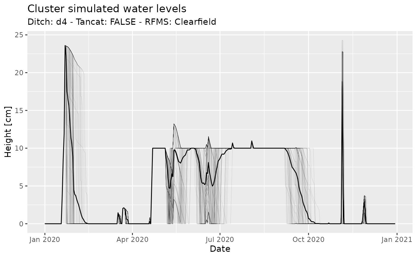
          paste("Ditch:", ditch, "- Tancat:", tancat, "- RFMS:", rfms_name)
          )

Further information

Further details will appear in this and possibly other vignettes. For specific problems, you can file an issue on Github.